
The inspiration for this article came after reading several articles by Scott Berry, former writer of the A Statistician Reads the Sports Page column. I found two of his articles particularly interesting. One discussed the dominance of Tiger Woods in golf using data from the beginning of the 1999 PGA Tour season through the 2001 Masters Tournament. The other focused on leisure sports such as bass fishing and darts. In both, a Bayesian hierarchical model (with a normal distribution for the data) was used to estimate the abilities of the golfers and the fishermen, as well as the difficulty of the tournaments in which they participated. I began to consider if there were any other sports, whether ?leisure? or ?athletic,? that had not been thoroughly investigated and whose data could be modeled in a similar fashion. The sport of ten-pin bowling immediately came to mind.
It appears there has been little research on bowling. In ?Quantitative Aspects of Five-Pin Bowling,? authors Wenjun Chen and Tim Swartz show that the logarithms of five-pin bowling scores are approximately normally distributed. In ?Bowlers? Hot Hands,? Reid Dorsey-Palmateer and Gary Smith investigate whether a ?hot hand? effect exists in professional bowling. Using data from the 2002?2003 Professional Bowlers Association (PBA) National Tour season, the authors find evidence that for some professional (ten-pin) bowlers, the probability of rolling a strike on the current frame is not independent of the outcomes on previous frames and that there is more variation in the number of strikes rolled across games than would be predicted by chance alone. In particular, they found that most bowlers were more likely to strike in the current frame if they had struck in the previous frame (or frames). These results provide evidence that the ?hot hand? effect exists in professional bowling.
As far as I know, however, there has been no attempt to model the scores of professional or recreational (ten-pin) bowlers. I attempt to do so in this article. In particular, I am interested in examining bowling data from tournaments played on the PBA National Tour. My primary goals are to estimate the variation in bowling scores, bowler abilities, and tournament difficulties. I also attempt to (via simulation) estimate the probabilities of top bowlers winning tournaments and the probabilities of non-exempt bowlers making it into tournaments through the tournament qualifying round (TQR).
The Game of Bowling and the PBA Tour
Bowling is a game in which a spherical ball (a ?bowling ball,? usually weighing between 10 and 16 pounds) is rolled down a lane approximately 60 feet long and 41.5 inches wide in an attempt to knock down as many pins as possible. (In ten-pin bowling, there are 10 pins arranged in a pyramid shape at the end of the lane.) Each lane is coated with oil that can be applied in a variety of ways, and it is these different oil patterns that have a major effect on how difficult it will be for bowlers to achieve high scores.
For instance, an easy oil pattern is when a lot of oil is applied to the middle of the lane and very little oil is applied to the outside of the lane (as is the case for a typical bowling alley that services bowlers of all skill levels).
The objective of the game is to knock down as many pins as possible in each of 10 separate frames. (These 10 frames constitute one game.) In each frame, a bowler is given two attempts to knock down all 10 pins, with a successful attempt on the first roll known as a ?strike? and a successful attempt on the second roll known as a ?spare.? A frame in which fewer than 10 pins are knocked down after two rolls is known as an ?open frame.? In the tenth and final frame, a bowler is given a chance to roll a third time if he or she is able to score a ?strike? or a ?spare? in that frame. Thus, in the tenth frame, it is possible to roll three strikes (as well as a strike and a spare or an open frame).
The scoring system, while not overly complex, will not be thoroughly explained here (although an example will be provided later). Basically, high scores are achieved when many strikes and/or spares are rolled consecutively, while open frames are detrimental to achieving a high score. The highest possible score is 300, which is accomplished when 12 consecutive strikes are rolled (one in each of the first nine frames and three in the tenth frame). The lowest possible score is 0, which results if no pins are knocked down in any of the 10 frames.
Due to their ability to roll many consecutive strikes and/or spares, elite bowlers are able to achieve scores of 200 or more in a game on a regular basis. For a comprehensive analysis of the scoring system, including the number of ways in which all 301 possible scores can be achieved (see reference).
The PBA Tour is the top professional tour for ten-pin bowling in the United States. It consists of several tours, including the national tour, regional tour, women?s series (which became defunct after the 2009?2010 season), and senior tour. The national tour is comprised of the best bowlers in the country, as well as many top bowlers from other countries. The regional tour is just below the national tour and consists of seven regions throughout the country.
Despite the distinction as the ?minor leagues? of professional bowling, many top professionals bowl in regional tour events to keep their skills sharp between tournaments on the national tour (and because prize money at the highest levels of bowling is nowhere near as lucrative as it is in other individual sports, such as golf). Despite the current lack of a women?s tour, many professional female bowlers compete in both PBA national and regional tour events. While both of these tours are predominately male, women have achieved a moderate amount of success in recent years. Finally, the senior tour is for professional bowlers over the age of 50.
Since the focus of this article is the PBA National Tour, it is worthwhile to examine this tour in more depth. For most of its history, tournaments on the PBA National Tour were open to the entire PBA membership. Beginning in October of 2004, however, the national tour changed to an all-exempt format. In this format, only 64 bowlers would compete in certain tournaments throughout the season, while most other tournaments would be open to the entire PBA membership (as well as non-members, on occasion). Those bowlers who earned exemptions for the upcoming season would automatically make the field of 64 in the relevant tournaments, while all remaining spots (usually between four and 12) would be filled by those bowlers who had the highest cumulative scores in the TQR. With this change in the format, it became (and remains) beneficial to earn an exemption for the upcoming season. (See the appendix in the supplemental material at http://chance.amstat.org/category/supplemental for a complete list of how exemptions can be earned.)
To become a PBA member, and therefore become eligible to earn an exemption on the national tour, a bowler must meet the following criteria:
- (1) Have an average score of 200 or higher for a minimum of 36 games in a United States Bowling Congress (USBC)-certified league or tournament club within the previous year
- (2) Have an average score of 190 or higher for a minimum of 36 games in a USBC-certified Sport Bowling League within the previous year
These same criteria also must be met for a bowler who is not a PBA member to be eligible to bowl in a PBA event (not just an event on the national tour). Thus, it is clear that only elite bowlers (relative to most people who bowl) are eligible to compete in PBA events, both at the national and regional levels.
Data Set and Model
The data for this analysis comes from tournaments that were contested on the PBA National Tour, which was available from the PBA. (In a few rare cases, data were cross-referenced with the website bowlingdigital.com). For each tournament, I recorded each bowler?s name (first and last), his or her scores for all games bowled, the oil pattern (or patterns) used by the tournament, and the name of the tournament.
For data to be collected from a tournament, scores for every bowler who competed in the tournament had to be available, including those who competed in the TQR. As it happened, this criterion was met for most tournaments that began after the inception of the all-exempt format in October of 2004. In all but two tournaments for which data were collected, every score from every round was available. The lone exceptions were the USBC Masters tournament that was played during the 2009?2010 season, for which I was only able to collect scores for the first three qualifying rounds and the final three matches of the tournament, and the Exempt Doubles Classic that was played during the 2007?2008 season, for which I was only able to collect scores for the first three rounds.
For two other doubles tournaments (for which each doubles team was mixed gender), I only collected individual scores in the early rounds of the tournament, and not for rounds where team members bowled together in the same games.
In total, there were 117 tournaments for which data were collected, beginning with the 2004?2005 season and going through the end of the 2009?2010 season. There was a total of 278,579 games bowled by 3,931 bowlers during these tournaments.
A major issue encountered during the data-collection process involved attributing scores to the correct bowlers. Since many of the bowlers had common names and a bowler?s name was not always recorded as the same name for every tournament (e.g., Mike or Michael, with or without a ?Jr.? after the last name, etc.), it was a painstaking process to comb through all the names and determine whether different names in different tournaments actually referred to the same person or if the same name was actually two or more people.
Since information about date of birth and/or place of residence was provided for most bowlers, it usually wasn?t too difficult to determine which scores to attribute to which bowlers. However, in a few cases, it was only possible to make an educated guess, and thus the total of 3,931 bowlers is probably not exactly correct, although it should be close to the actual number.
There was also a minor issue with determining which scores were actually ?believable? as opposed to incorrectly recorded or as the result of fewer than 10 frames being bowled. For instance, a bowler was given a score of zero in some cases. These scores were not recorded, as they are almost certainly a result of the bowler either withdrawing from the tournament or being penalized for some infraction. In a few rare cases, low non-zero scores were given, and an educated guess was made to determine whether to record them. Given the size of the data set, it is believed that the results of the analysis would change little no matter what decisions were made concerning the few games in question.
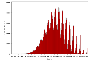
Figure 1. Histogram of bowling scores on the PBA Tour
The data for this histogram consist of scores for 278,579 games bowled by 3,931 bowlers over 117 tournaments on the PBA National Tour beginning in the 2004?2005 season and going through the 2009?2010 season (single-pin intervals).
A histogram of all 278,579 scores in the data set is presented in Figure 1. The histogram displays frequencies for each individual score, with each score represented by a thin bar. The mean of all scores was approximately 205.65, with a standard deviation of 31.91. There were 37 scores below 100 (with a low score of 78) and 555 perfect scores of 300.
The shape of the distribution is odd, with many peaks and valleys, especially for scores above 170. Most of the peaks occur at higher scores in ten-pin intervals (e.g., 171?180, 181?190, etc.), while the valleys appear at lower scores in the same ten-pin intervals. This is likely attributable to elite bowlers typically knocking down either nine or 10 pins (and rarely fewer than six) on their first roll of a frame. For example, to achieve a score in the 291?300 range, a bowler must successfully strike on his or her first 11 rolls (i.e., strikes in the first nine frames and on the first two rolls in the tenth frame). On the 12th and final roll, it is unlikely that an elite bowler will only knock down a few pins, and thus almost all of the scores in the 291?300 range are either 299 or 300.
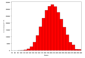
Figure 2. Histogram of bowling scores on the PBA Tour (10?pin intervals)
The data for this histogram consist of scores for 278,579 games bowled by 3,931 bowlers over 117 tournaments on the PBA National Tour beginning in the 2004?2005 season and going through the 2009?2010 season (ten-pin intervals).
Clearly, the distribution of bowling scores in Figure 1 is not normally distributed, but it is fairly symmetrical, with slight positive skew (indicating a slightly longer right tail than the normal distribution) and negative kurtosis (meaning scores in the tails of the distribution have lower probability of occurring than would be predicted by the normal distribution). Due to this approximate symmetry and because most ten-pin intervals have a similar shape, I decided to check the distribution of the bowling scores when they were grouped into ten-pin intervals (e.g., 71?80, 81?90, ?, 291?300). The histogram of these grouped scores is presented in Figure 2.
The distribution is approximately normally distributed (again with slight positive skew and negative kurtosis). Therefore, while the normal distribution would certainly over-predict the probability of achieving a lower score in a given ten-pin interval and under-predict the probability of achieving a higher score in the same ten-pin interval, these predictions are similar across each ten-pin interval, thus it seems likely that a bowler?s average could be estimated relatively accurately using a normal distribution. The same can be said of estimating the average difficulty of a tournament based on all games bowled in that tournament. Because the normal distribution appears to be reasonable for predicting a bowler?s true average and the average difficulty of a tournament, it was used to model the bowling scores in the data set.
The model I use for bowling scores is similar to Berry?s model for golf scores. Like Berry?s model, two particular aspects of the data I attempt to capture with my model are varying difficulties of tournaments and regression to the mean. The following model controls for these particular aspects: Let ?i be the intrinsic ability of the ith bowler (assumed to be constant for each bowler over the time period for which I have collected data), which, in this case, can be interpreted as the ith bowler?s average score in an average PBA National Tour tournament. Let ?j be the intrinsic difficulty of the ith tournament, where the value for each ? represents each tournament?s deviation in score from the average tournament value of 0. Therefore, difficult tournaments will have negative values of ? and easier tournaments will have positive values of ?. Typically, the factor that has the biggest effect on a tournament?s difficulty is the oil pattern, but there also could be factors such as tournament location, lane material, and bowling pin material. Each bowler?s estimated average score in a particular tournament is based on the values of these two parameters, which can be expressed in the following manner:
- ?ij = ?i + ?j
- yij ~ Normal(?ij,?)
In the notation above, yij represents the score for the ith bowler in the jth tournament, while ? can be interpreted as the standard deviation from each bowler?s average score. In this model, the bowler abilities and tournament difficulties are additive, thus a bowler?s average score will rise or fall depending on the difficulty of the tournament. For example, if a bowler?s average score in an average tournament is 200 (i.e., ? = 200), then his expected average in a tournament with ? = -5 is 195 and his expected average in a tournament with ? = 5 is 205. For those interested in how the values of the parameters are estimated, see the appendix in the supplemental material.
I previously mentioned that the model attempts to capture phenomena known as ?regression to the mean.? In the context of bowler abilities (i.e., the ??s in the model specification), this means a given bowler?s ability is ?regressed? toward the average ability of all bowlers. The factors that influence how much a given bowler?s ability is regressed are the distance from the average ability, the total number of games bowled, and the difficulty of the tournaments in which a bowler competes.
Regressing bowlers toward the mean makes intuitive sense because we naturally expect a bowler who has a high average but only a relatively small number of games bowled to not be as good as his average indicates (and vice-versa). It is more likely that he simply bowled well for those few games and that his average after bowling many games would be lower.
For example, the bowler with the highest average in the data set is Jack Ness, who compiled a 236.17 average in 24 games at the Pepsi Red, White, and Blue Open during the 2009?2010 season. While this is impressive, it was only the 19th-highest average in the tournament, with the winner achieving an average of 247.16. Also, I do not believe many people would consider Ness?s 236.17 average in 24 games to be more impressive than, for example, Walter Ray Williams Jr.?s average of 225.07 (17th-highest among all bowlers) in 2,889 games, even if both players bowled all their games in the same tournament. Thus, the structure of the model regresses the ability of players such as Ness appropriately. For details about the model, refer to the supplemental material
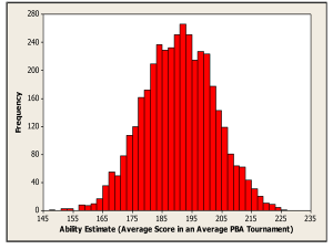
Figure 3. Histogram of ability estimates for 3,931 bowlers in 117 PBA tournaments (2004?2005 through 2009?2010 seasons)
Results for Bowler Abilities and Tournament Difficulties
A histogram of all 3,931 bowler ability estimates ??s) is displayed in Figure 3. (Each bar represents a two-pin interval.) The ability estimate for the average bowler (call this estimate ?average) was 190.69 (sd = 0.74) and the standard deviation for all bowler ability estimates (call this estimate ?) was 13.35 (sd = 0.19). Therefore, the average score for an average bowler in an average PBA tournament is 190.69, and it is clear from Figure 3 (and the value of ?) that there is substantial variation in bowler abilities. Notice also that the ability estimate for the average bowler is appreciably lower than the average of all 278,579 scores in the data set (which was about 205.65). This is due to many more games being bowled by the higher-ranked bowlers than by the average- and lower-ranked bowlers, which led to an inflated average for the actual scores relative to the ability estimate for the average bowler.
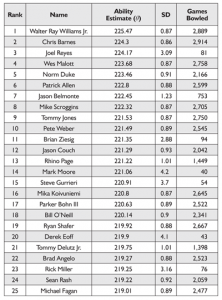
Table 1?List of the Top 25 Bowlers by Ability
Table 1 lists the 25 bowlers with the highest ability estimates, along with their corresponding standard deviations and total number of games bowled. As is evident from the table, players who have bowled fewer games have larger standard deviations because their true abilities are much less certain. Because the ability estimates are assumed to come from a normal distribution, an approximate 95% credible interval (which is a Bayesian interval estimate whose computation and interpretation is different than that of the classic ?confidence interval?) can be constructed by taking the ability estimate plus or minus two times the standard deviation. For example, the approximate 95% credible interval for the highest-ranked bowler, Williams Jr., is given by 225.47?(2*0.87) = (223.73, 227.21). The interpretation of this interval is that there is a 95% probability that Williams Jr.?s true ability (his average score in an average PBA tournament) is between 223.73 and 227.21.
Bowling fans will recognize most of the names on this list. Williams Jr. is considered by many to be the greatest bowler of all time. Chris Barnes is considered by many fans and fellow professionals to be the best bowler in the game today, having won at least $100,000 in his last eleven seasons on tour. The 3rd-ranked bowler, Joel Reyes, is likely unfamiliar to most bowling fans, and, indeed, I was surprised to see him ranked so high by the model. With so few games bowled compared to the rest of the bowlers in the top 10, I was initially curious why he wasn?t regressed more strongly toward the average bowler. (His average in 81 games over three tournaments was 227.74). I believe the answer lies in the fact that his 81 games bowled puts him in the 89.6th percentile for all bowlers in the data set (the median number of games bowled is 18). So while he has few games bowled relative to many of the better-known bowlers, he has bowled more games than a significant majority of the other bowlers in the data set, and therefore his ability estimate was not regressed too much. This is a likely explanation for why the other five bowlers with fewer than 100 games bowled appear in the top 25 as well.
Finally, note that Jack Ness is not among the top 25 bowlers listed in Table 1. Given that the tournament he bowled in was the easiest of all 117 and because he only bowled 24 games, Ness finished as the 125th-ranked bowler with ? = 212.81 and a standard deviation of 5.21.
Because bowling is one of the few sports in which female professionals can legitimately compete with their male counterparts, I was interested to see where the top female bowlers were ranked. The top three were Liz Johnson (83rd, ? = 214.57, sd = 1.16), Kelly Kulick (114th, ? = 213.13, sd = 1.24), and Carolyn Dorin-Ballard (119th, ? = 213, sd = 1.83).
Johnson was voted the female bowler of the decade for 2000?2009 in a poll by US Bowler magazine. Kulick is the only woman to ever win a PBA National Tour event (Tournament of Champions in the 2009?2010 season) and earn an exemption (2006?2007, 2010?2011, and 2011?2012 seasons). She placed third in the same poll by US Bowler magazine. Dorin-Ballard had a successful career on the now defunct Professional Women?s Bowling Association (PWBA) Tour, winning 20 titles in 14 years. She placed second in the poll by US Bowler.
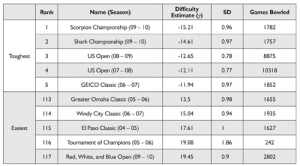
Table 2?List of the Five Toughest and Five Easiest PBA Tournaments by Difficulty
Table 2 lists the five toughest and five easiest tournaments by their difficulty estimates (??s), along with their corresponding standard deviations and total number of games bowled. Just like the bowler ability estimates, tournaments with fewer games bowled have larger standard deviations and are regressed toward the mean more strongly. (The average tournament difficulty is 0.) Once again, an approximate 95% credible interval can be constructed by taking the difficulty estimate plus or minus two times the standard deviation. The standard deviation for all tournament difficulty estimates was 7.49 (sd = 0.5), indicating there is considerable variation in the difficulties of the tournaments.
It was interesting to see how tournament difficulties varied by season and oil pattern. In general, tournaments in the most recent seasons were more difficult. The 2009?2010 season was especially difficult, as six of the 10 most difficult tournaments were played during that season. I also found it intriguing that tournaments that used the same oil pattern sometimes differed dramatically in difficulty. For example, the Scorpion Championship (which uses a ?scorpion? oil pattern) that was played during the 2008?2009 season was one of the easiest tournaments in the data set (110th, ? = 11.98, sd = 0.94), while the same tournament played the following season was the most difficult (see Table 2). The PBA did make major changes to several oil patterns prior to the 2009?2010 season, however, so perhaps such a colossal change in difficulty is not so surprising. But, even within the same season, there was sometimes a significant disparity in the difficulties of tournaments that used the same oil pattern, indicating that either factors other than the oil pattern play a major role in determining a tournament?s difficulty and/or different tournaments can apply the same oil pattern to the bowling lanes in vastly different ways.
Probabilities for Individual Bowler Match-Ups and Tournaments
One of the reasons a normal distribution was used to model the bowling scores is because it allows for relatively easy computation of probabilities via the use of the standard normal cumulative distribution function, denoted by ?. However, this ease of computation is only meaningful if the normal distribution fits the data reasonably well. As previously mentioned, the individual bowling scores are clearly non-normal (see Figure 1), but the distribution of scores using ten-pin intervals is approximately normally distributed (see Figure 2). Therefore, a bowler?s average is likely to be accurately estimated by the normal distribution, which allows for relatively accurate calculation of probabilities for individual bowler match-ups and tournaments with many bowlers.
To calculate the relevant probabilities, we need to know the value of ? from the model specification that was presented earlier. Recall that ? is the standard deviation from each bowler?s average score, which is assumed to be the same for all bowlers. The estimate for the value of ? was 27.47 (sd = 0.04). I suspect most bowling fans are not surprised by this estimate, since bowling scores can vary dramatically from one game to the next. This high variation is due in large part to the scoring system in bowling. I illustrate this with a hypothetical example, which is shown in Figure 4.

Figure 4. Sample bowling score
In this example, a strike is indicated by an X and a spare is indicated by a /. The final score for this game is 246. Now suppose the eight pins that were knocked down on the first roll in the eighth frame resulted in a split (a situation in which achieving a spare is difficult). Let?s assume one pin is knocked down on the next roll in the eighth frame and nothing else changes. Now the score for this game is 235. Now, let?s assume that, in addition to the open frame in the eighth, the fourth frame results in nine pins being knocked down on the first roll followed by a spare. The score for this game now becomes 224. If we further assume one of the spare conversions is missed, say the spare attempt in the seventh frame, then the score drops to 214. This example should give those who are unfamiliar with the scoring system in bowling an indication of how big of an effect a few pins can have on a bowler?s final score.
As a check of the validity of the normal distribution for probabilistic purposes, several bowler match-ups were simulated using their estimated abilities and the estimated value of ? = 27.47. The results were compared with simulations using each bowler?s empirical distributions (i.e., each bowler?s actual scores). Those bowlers who had many games bowled in the data set were chosen for the comparisons because their empirical distributions are much more reflective of their true score distributions (i.e., they have bowled enough games to achieve a variety of scores).
A particular comparison was between Williams Jr. and Barnes, the two bowlers with the highest ability estimates (see Table 1). Each of their individual score distributions closely resembled the distribution of scores in Figure 1 (except that both were shifted to the right), and each of their score distributions were approximately normally distributed (closely resembling Figure 2) when they were grouped into ten-pin intervals. Four match lengths (of 1, 3, 5, and 7 games) were simulated 10 million times using both the normal distribution estimates and empirical distributions (with scores constrained between 0 and 300). Each simulation recorded which player won the match and the total scores for each player at the end of each match. Therefore, in addition to calculating the probability of each player winning a particular match, the probability of each player winning a match with the highest cumulative score was calculated.
I decided to calculate this second probability because it is not uncommon for a bowler to have a higher cumulative score and still lose the match (assuming the match is longer than one game) due to a bowler having to win more individual games to win a match (i.e., be the first to win two games in a three-game match, three games in a five-game match, etc.). For the match-up between Williams Jr. and Barnes, the simulations produced the results in Table 3, with the probability of Barnes winning with the highest cumulative score in parenthesis.

Table 3?Comparison of Probabilities in a Match of Various Lengths Between Walter Ray Williams Jr. and Chris Barnes Using the Normal and Empirical Distributions for Their Bowling Scores
Clearly, the probabilities of winning the match and winning the match with the highest cumulative score are close between the normal distribution estimates and the empirical distributions. Comparisons between other bowlers resulted in similar agreement.
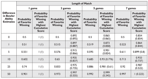
Table 4?Probabilities of Superior Bowler Winning a Match of Various Lengths and Winning with the Highest Cumulative Score (Probability of Underdog Winning with Highest Cumulative Score in Parentheses)
Table 4 presents simulated results for selected differences in bowler ability estimates with ? = 27.47. Note that the probabilities of the superior bowler winning (?favorite? in the table) can be calculated by using the standard normal cumulative distribution function, denoted by ?. (I chose to simulate because I wanted to estimate the probabilities of each player winning with the highest cumulative score as well). For example, when the difference in bowler ability estimates is five pins, the probability of the superior bowler winning a one-game match is ?(5/(27.47*?2))?0.551, which is in agreement with Table 4.
As expected, the probability of the favorite winning increases as the number of games in the match increases. However, the probabilities listed in Table 4 make it clear that the high variation in bowling scores has a major effect on the outcome of a particular bowling match. Even when the average scores between two players differ by 50 pins, the weaker bowler still has a 10% probability of winning in a one-game match.
It is also noteworthy how the probability of the favorite (and underdog) winning the match with the highest cumulative score changes as the difference in bowler abilities and number of games change. When the difference in bowler abilities is less than 10 pins, the probability of the favorite winning with the highest cumulative score decreases as the number of games increases, but the pattern reverses for differences in bowler abilities above 10 pins. Not surprisingly, the probability of the underdog winning with the highest cumulative score decreases steadily as the difference in bowler abilities increases and the number of games increases.
In addition to individual match-ups, it is also interesting to consider the probabilities of bowlers winning tournaments or advancing from the TQR. On the PBA National Tour, there are typically two types of tournaments: match-play and step-ladder. In a match-play tournament, 64 players (comprised of exempt players and those who advance from the qualifying round) play in a bracket-style format in which 32 matches of a certain length (usually seven games) take place in the first round (#1 vs. #64, #2 vs. #63, ?, with the winners moving on to the next round), 16 matches take place in the next round (again, the winners move on), ?, all the way to the final match, in which the winner is declared the winner of the tournament.
Over the past few seasons, the match-play format has typically begun with 32 players who advance from the original field of 64 based on highest cumulative scores after bowling a certain number of games.
In a step-ladder tournament, all players in the field (whether restricted to 64 or open to any number who qualify to compete) bowl a certain number of games in the initial round and the field is arbitrarily cut to a number of players who achieved the highest cumulative scores afterward. This process continues in subsequent rounds until the match-play round is reached. In this round, each player competes in one-game matches against as many other players as possible, with an additional 30 pins added to the cumulative score of the winner and 15 pins added for a tie (cumulative scores carry over from the initial rounds).
The last match for all players in the match-play round is typically called the ?position round,? and in this case, players who are close in cumulative score play against one another (i.e., the player with the highest cumulative score plays the player with the second-highest cumulative score, etc.). At the conclusion of the match-play round, usually the four or five players with the highest cumulative scores move on to the step-ladder finals. When five players move on, the first one-game match takes place between the player with the fifth-highest cumulative score and the player with the fourth-highest cumulative score. The winner of this match then competes in a one-game match against the player with the third-highest cumulative score, with the winner moving on to play the player with the second-highest cumulative score. Finally, whoever has made it to the final one-game match competes against the player with the highest cumulative score, and the winner of that match wins the tournament.
Having already investigated individual match-ups (see Table 4), I chose to examine a step-ladder tournament using the 64 players with the highest ability estimates. I used a common format for this type of tournament that has been used in recent seasons on the PBA Tour. Under this format, 64 players bowl 14 games each in the first round, after which the players with the 32 highest cumulative scores move on to the second round. In this round, each of the remaining 32 players bowls nine more games, after which the field is cut to 16 players. These remaining 16 players bowl nine games, and, at the end of this round, the five players with the highest cumulative scores (after the previous 32 games) move on to the step-ladder finals, which proceeds as described above. (I ignore the additional 30- or 15-pin bonuses awarded in the match-play round.)
Using this format with the top 64 bowlers and simulating the tournament 1 million times (using each bowler?s ability estimate and ? = 27.47), the top 10 bowlers (see Table 1) have the following probabilities of winning the tournament: 0.054, 0.044, 0.043, 0.039, 0.037, 0.032, 0.03, 0.03, 0.025, and 0.025. For comparison, the 64th-ranked bowler has a probability of 0.006 of winning the tournament. Considering the large variation in bowling scores and high quality of the field, I think Williams Jr.?s 5.4% probability of winning the tournament (which corresponds to odds against winning of about 17.5 to 1) is pretty remarkable. Even so, it is clear that the large variation in bowling scores gives many of the top 64 bowlers a legitimate chance to win the tournament.
One other tournament simulation I was interested in conducting was the probability of advancing from the TQR into the field of 64 for bowlers of various abilities. I decided to calculate three sets of probabilities for varying strengths of the qualifying field. In each case, there were 80 bowlers in the field, eight qualifying spots were available, and each player bowled seven games.
The ?strong? field consisted of the top 40 bowlers below the top 56 who were already exempt (i.e., those bowlers who were ranked 57th through 96th, whose values range from 215.98 to 213.86), 20 bowlers who were all one standard deviation above average (thus, each of these 20 bowlers had ?above_average= ?average+ ?=190.69 + 13.35 = 204.04), 15 average bowlers (?average=190.69 ), and five bowlers who were all one standard deviation below average (?below_average= ?average ? ? = 190.69 ? 13.35 = 177.34).
The ?average? field consisted of the top 30 bowlers below the top 56 who were exempt, 20 bowlers one standard deviation above average, 20 average bowlers, and 10 bowlers one standard deviation below average.
Finally, the ?weak? field consisted of the top 20 bowlers below the top 56 who were exempt, 20 bowlers one standard deviation above average, 20 average bowlers, and 20 bowlers one standard deviation below average.
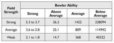
Table 5?Odds to 1 Against Advancing from the TQR for Various Field Strengths and for Bowlers of Various Abilities, Assuming a Field Size of 80 Bowlers, 8 Qualifying Spots, and 7 Games Bowled for Each Bowler
Using these ability estimates and ? = 27.47, all three tournaments were simulated 1 million times. The range of the odds against advancing to the field of 64 for the strong bowlers (those right below the top 56 exempt) and the average odds against advancing to the field of 64 for the other three groups of bowlers are presented in Table 5.
As expected, the table indicates that as the field gets weaker, every bowler becomes more likely to advance from the qualifying round into the field of 64. It is also not surprising that bowlers of below average ability are extremely unlikely to make it out of the qualifying round. Bowlers of average ability also do not often make it out of the qualifying round, while bowlers of above average ability have a small but realistic chance of qualifying for the field of 64. Although the strong bowlers are by far the most likely to make the field of 64, it is by no means certain that they will do so. Even in a weak field, the best bowlers will only qualify for the tournament between 32% and 36% of the time. I believe these results demonstrate just how beneficial it is to earn an exemption on the PBA National Tour.
Conclusion
The primary focus of this article has been estimating different sources of variation in bowling. As expected, the natural variation in bowling scores was found to be quite high (? = 27.47), and because of this substantial variation, it is unlikely that any model would be able to predict bowling scores with relatively little error. Despite this, there also appears to be considerable variation in bowler abilities and tournament difficulties (standard deviations of 13.35 and 7.49, respectively).
In his article on golf scores, Berry estimated the standard deviation of golf scores at 3.12 and the standard deviation of golfer abilities at 2.1, which results in a standard deviation of score to standard deviation of ability ratio of approximately 1.49. This ratio is slightly higher in bowling, at approximately 2.06. I actually expected the ratio in bowling to be much higher than the ratio in golf and was pleasantly surprised to find that the two ratios were not incredibly different. Given that golf is perceived as a game that requires great skill to perform well, I think the similarities in natural variation in score to variation in ability ratios give credence to the belief that bowling is also a game that requires tremendous skill to perform well.
Perhaps the strangest result found was that tournaments using the same oil pattern occasionally differed significantly in difficulty. There were a few tournaments that consistently used the same oil pattern and were often similar in difficulty, but this similarity was nonexistent for other tournaments. As previously explained, part of the discrepancy is likely due to the oil patterns sometimes undergoing modifications, although it is difficult to determine how dramatically these changes should affect performance. While I still believe a tournament?s oil pattern has the most significant influence on it?s difficulty, perhaps a future analysis could investigate other factors that might affect the difficulty of a given tournament.
Finally, it is worth noting that all the tournaments for the 2010?2011 season on the PBA National Tour (which have been significantly reduced in number relative to previous seasons) will use the step-ladder format, as opposed to the match-play format. It also appears that the 2010?2011 season has fewer tournaments using the 64-player, all-exempt format.
While it is difficult to say whether these changes will become permanent, I believe the step-ladder format is advantageous for superior bowlers, while allowing more competitors is a disadvantage for superior bowlers (unless the number of games bowled before each cut is increased). I am interested in seeing if and how the tournament structure of the PBA National Tour changes in the coming years, as well as who benefits if changes are implemented.
Back to Top
Further Reading
Berry, S.M., C.S. Reese, and P.D. Larkey. 1999. Bridging different eras in sports. Journal of the American Statistical Association 94:661?686.
Berry, S.M. 2001. How ferocious is Tiger? CHANCE 14:51?56.
Berry, S.M. 2002. Read during your leisure time. CHANCE 15:48?55.
Chen, W., and T. Swartz. 1994. Quantitative aspects of five-pin bowling. Journal of the American Statistical Association 48:92?98.
Dorsey-Palmateer, R., and G. Smith. 2004. Bowlers? hot hands. The American Statistician 58:38?45.
Kruschke, J.K. 2011. Doing Bayesian data analysis. Academic Press: Massachusetts.
Ntzoufras, I. 2009. Bayesian modeling using WinBUGS. John Wiley & Sons: New Jersey.
Wikipedia Contributors. Ten-pin bowling. Wikipedia, The Free Encyclopedia. http://en.wikipedia.org/wiki/Ten-pin_bowling
Source: http://chance.amstat.org/2011/09/professional-bowling/
camelot brooklyn contact ocean city maryland baklava msp 101
No comments:
Post a Comment
Note: Only a member of this blog may post a comment.